41 add data labels to pivot chart

Add a DATA LABEL to ONE POINT on a chart in Excel All the data points will be highlighted. Click again on the single point that you want to add a data label to. Right-click and select ' Add data label '. This is the key step! Right-click again on the data point itself (not the label) and select ' Format data label '. You can now configure the label as required — select the content of ... How to Add Data Labels in Excel - Excelchat | Excelchat After inserting a chart in Excel 2010 and earlier versions we need to do the followings to add data labels to the chart; Click inside the chart area to display the Chart Tools. Figure 2. Chart Tools. Click on Layout tab of the Chart Tools. In Labels group, click on Data Labels and select the position to add labels to the chart.

Add & edit a chart or graph - Computer - Google Docs Editors Help Double-click the chart you want to change. At the right, click Customize. Click Gridlines. Optional: If your chart has horizontal and vertical gridlines, next to "Apply to," choose the gridlines you want to change. Make changes to the gridlines. Tips: To hide gridlines but keep axis labels, use the same color for the gridlines and chart background.

Add data labels to pivot chart

Dynamically Label Excel Chart Series Lines • My Online ... Sep 26, 2017 · Great question. Pivot Charts won’t allow you to plot the dummy data for the label values in the chart as it wouldn’t be part of the source data, so the options are: 1. create a regular chart from your PivotTable and add the dummy data columns for the labels outside of the PivotTable. Not ideal if you’re using Slicers. Excel charts: add title, customize chart axis, legend and data labels Click anywhere within your Excel chart, then click the Chart Elements button and check the Axis Titles box. If you want to display the title only for one axis, either horizontal or vertical, click the arrow next to Axis Titles and clear one of the boxes: Click the axis title box on the chart, and type the text. Copy a Pivot Table and Pivot Chart and Link to New Data Jul 15, 2010 · -the pivot chart, or the pivot table, or both, are moved into another sheet (the chart with cut-paste, pivot with the option-Move Pivot Table) This action, of moving the chart or pivot table will add an absolute path to the data source : ‘Book1 only pivot table.xlsx’!Table1

Add data labels to pivot chart. Pivot Chart Data Label Help Needed - Microsoft Community Open the Excel file with Pivot Chart and enabled with Data Labels> Click on the Labels displayed in the Chart> Right-click> Click Format Data Labels> Label Options> Number> In the Category, select the format as per your requirement. Here is the reference article: Change the format of data labels in a chart. Change the format of data labels in a chart To get there, after adding your data labels, select the data label to format, and then click Chart Elements > Data Labels > More Options. To go to the appropriate area, click one of the four icons ( Fill & Line, Effects, Size & Properties ( Layout & Properties in Outlook or Word), or Label Options) shown here. Data Labels in Excel Pivot Chart (Detailed Analysis) Adding Data Labels in Pivot Chart — To do this, go to Insert tab > Tables group. · Then in the dialog box, select the range of cells of the primary ... How to Add Filter to Pivot Table: 7 Steps (with Pictures) Mar 28, 2019 · The attribute should be one of the column labels from the source data that is populating your pivot table. For example, assume your source data contains sales by product, month and region. You could choose any one of these attributes for your filter and have your pivot table display data for only certain products, certain months or certain regions.

Overview of PivotTables and PivotCharts PivotCharts display data series, categories, data markers, and axes just as standard charts do. You can also change the chart type and other options such as the titles, the legend placement, the data labels, the chart location, and so on. Here's a PivotChart based on the PivotTable example above. For more information, see Create a PivotChart. How to update or add new data to an existing Pivot Table in Excel And here's the resulting Pivot Table: Change the Source Data for your Pivot Table. In order to change the source data for your Pivot Table, you can follow these steps: Add your new data to the existing data table. In our case, we'll simply paste the additional rows of data into the existing sales data table. How to Add Data to a Pivot Table: 11 Steps (with Pictures) - wikiHow You can do this in both Windows and Mac versions of Excel. Steps Download Article 1 Open your pivot table Excel document. Double-click the Excel document that contains your pivot table. It will open. 2 Go to the spreadsheet page that contains your data. Click the tab that contains your data (e.g., Sheet 2) at the bottom of the Excel window. 3 Create Dynamic Chart Data Labels with Slicers - Excel Campus You basically need to select a label series, then press the Value from Cells button in the Format Data Labels menu. Then select the range that contains the metrics for that series. Click to Enlarge Repeat this step for each series in the chart. If you are using Excel 2010 or earlier the chart will look like the following when you open the file.

How to change/edit Pivot Chart's data source/axis ... - ExtendOffice Step 1: Select the Pivot Chart you will change its data source, and cut it with pressing the Ctrl + X keys simultaneously. Step 2: Create a new workbook with pressing the Ctrl + N keys at the same time, and then paste the cut Pivot Chart into this new workbook with pressing Ctrl + V keys at the same time. Step 3: Now cut the Pivot Chart from ... Add or remove data labels in a chart - support.microsoft.com To label one data point, after clicking the series, click that data point. In the upper right corner, next to the chart, click Add Chart Element > Data Labels. To change the location, click the arrow, and choose an option. If you want to show your data label inside a text bubble shape, click Data Callout. How to Customize Your Excel Pivot Chart Data Labels - dummies The Data Labels command on the Design tab's Add Chart Element menu in Excel allows you to label data markers with values from your pivot table. When you click the command button, Excel displays a menu with commands corresponding to locations for the data labels: None, Center, Left, Right, Above, and Below. How to Make a Pie Chart in Excel & Add Rich Data Labels to The Chart! 8) With the one data point still selected, right-click this data point, and select Add Data Label>Add Data Callout as shown below. 9) Select only this data label and right-click and choose Insert Data Label Field as shown below. 10) Select [Cell] Choose Cell from the options.

31 Excel Chart Label Axis - Label Design Ideas 2020

Add Value Label to Pivot Chart Displayed as Percentage I have created a pivot chart that "Shows Values As" % of Row Total. This chart displays items that are On-Time vs. items that are Late per month. The chart is a 100% stacked bar. I would like to add data labels for the actual value. Example: If the chart displays 25% late and 75% on-time, I would like to display the values behind those %'s ...

How to hide zero value rows in pivot table?

Add vertical line to Excel chart: scatter plot, bar and line ... May 15, 2019 · Right-click anywhere in your scatter chart and choose Select Data… in the pop-up menu. In the Select Data Source dialogue window, click the Add button under Legend Entries (Series): In the Edit Series dialog box, do the following: In the Series name box, type a name for the vertical line series, say Average.

excel vba - VBA Pivot Chart data labels not appear - Stack Overflow

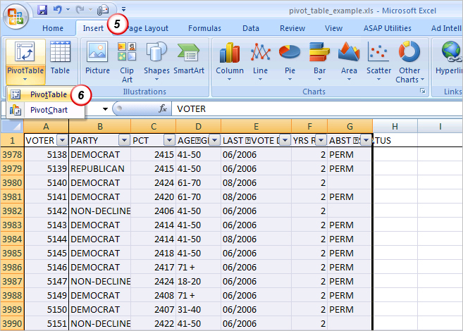
Automatic Row And Column Pivot Table Labels - How To Excel At Excel Select the data set you want to use for your table The first thing to do is put your cursor somewhere in your data list Select the Insert Tab Hit Pivot Table icon Next select Pivot Table option Select a table or range option Select to put your Table on a New Worksheet or on the current one, for this tutorial select the first option Click Ok

microsoft excel - How to add custom columns to Pivot Table (similar to Grand Total)? - Super User

Pivot Chart Formatting Changes When Filtered - Peltier Tech Apr 07, 2014 · I have a pivot chart based on data collected from a customer survey for 5 different customer bases (EUROPE, SOUTH AMERICA, ASIA, etc). The pivot chart will reference the same 5 bases each time, but with a different subject. For example: Satisfaction with Promotional Material, Satisfaction with Innovation of Products, etc.

In Search of the Elusive Pivot Table | Dynamic Edge, Inc. | Beyond Tech Support Dynamic Edge ...

Adding Data Labels to a Chart Using VBA Loops - Wise Owl To do this, add the following line to your code: 'make sure data labels are turned on. FilmDataSeries.HasDataLabels = True. This simple bit of code uses the variable we set earlier to turn on the data labels for the chart. Without this line, when we try to set the text of the first data label our code would fall over.

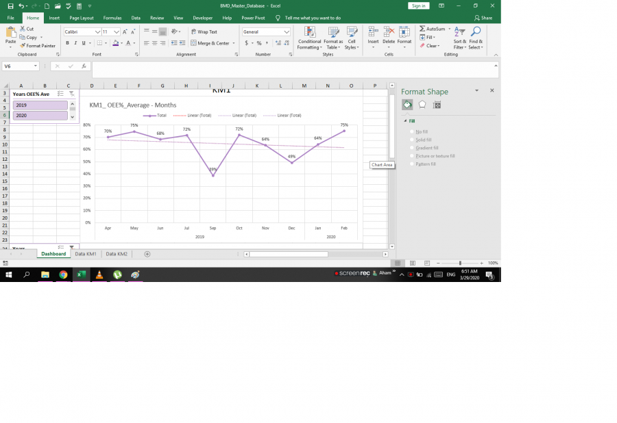
How to add the average baseline for a specific pivot chart | Dashboards & Charts | Excel Forum ...

Pivot Charts with Data Labels other than Values Click on data labels and use the right "arrow" to select that you want the information to appear above the bar. Then right click on the data label and select Format Data Labels, Under label options you have choices like Series name, Category name, etc. One spreadsheet to rule them all. One spreadsheet to find them.

» Excel Charts: Creating Custom Data Labels

How to add data labels from different column in an Excel chart? Right click the data series in the chart, and select Add Data Labels > Add Data Labels from the context menu to add data labels. 2. Click any data label to select all data labels, and then click the specified data label to select it only in the chart. 3.

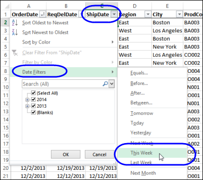
Dynamic Date Range Filters in Pivot Table – Excel Pivot Tables

How to make row labels on same line in pivot table? - ExtendOffice Please do as follows: 1. Click any cell in your pivot table, and the PivotTable Tools tab will be displayed. 2. Under the PivotTable Tools tab, click Design > Report Layout > Show in Tabular Form, see screenshot: 3. And now, the row labels in the pivot table have been placed side by side at once, see screenshot:

Share :